Parallel Computing

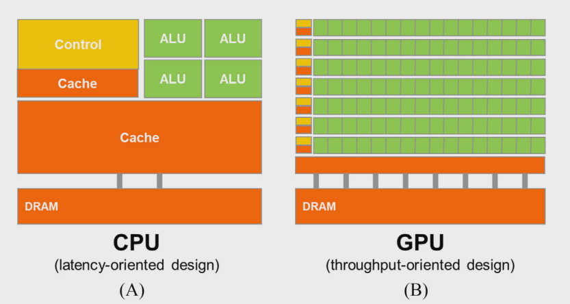
CPU and GPU Design Philosophies

The latency-oriented design of CPUs is highly advantageous for sequential operations and workloads that require low parallelism. By reducing execution latency for individual threads, CPUs excel in single-threaded performance and complex tasks involving conditional logic or frequent data accesses. However, this design approach comes with trade-offs: it demands significant chip area and power consumption to support advanced arithmetic units, large caches, and sophisticated control logic. This focus limits the CPU’s ability to handle highly parallel workloads efficiently, as the resources could have been used to include more arithmetic units or memory access channels.

In contrast, GPUs are designed for parallelism, making them more suitable for workloads involving a large number of threads but less optimized for minimizing latency in individual operations. Graphics applications require massive floating-point calculations and memory access, with performance often limited by data transfer rates. GPUs excel at handling large data movement in DRAM and leverage a relaxed memory model to support massive parallelism, crucial for high-quality video rendering.

Reducing latency is much more costly than increasing throughput when considering power and chip area. For example, doubling arithmetic throughput requires doubling the number of arithmetic units, which results in a proportional increase in chip area and power consumption. In contrast, halving latency often involves doubling the current, leading to a more than twofold increase in chip area and a fourfold increase in power consumption. Consequently, throughput optimization is generally a more resource-efficient design choice compared to latency reduction.

GPUs allow for longer latencies in their design, enabling savings in chip area and energy. This allows for the inclusion of more hardware units, thereby increasing overall processing capacity. In contrast, CPUs are optimized for low latency, but this comes at the cost of more limited parallelism. These two design approaches offer distinct advantages tailored to different needs.

Throughput-Oriented Design

The application software for these GPUs is expected to be written with a large number of parallel threads. The hardware takes advantage of the large number of threads to find work to do when some of them are waiting for long-latency memory accesses or arithmetic operations. Small cache memories in Fig. 1B are provided to help control the bandwidth requirements of these applications so that multiple threads that access the same memory data do not all need to go to the DRAM. This design style is commonly referred to as throughput-oriented design, as it strives to maximize the total execution throughput of a large number of threads while allowing individual threads to take a potentially much longer time to execute.

Compute Unified Device Architecture (CUDA)

GPUs are optimized for parallel, throughput-oriented tasks, while CPUs excel at low-latency, sequential operations. CPUs outperform GPUs in programs with few threads, whereas GPUs excel in programs with many threads. Consequently, many applications leverage both, running sequential tasks on CPUs and computation-intensive tasks on GPUs.

NVIDIA’s CUDA, introduced in 2007, facilitates joint CPU-GPU execution for such applications. The introduction of CUDA unlocked the parallel computing potential of GPUs for a broader developer audience. By removing graphics-based limitations, it enabled the use of GPUs in diverse fields such as scientific computing, artificial intelligence, and image processing. This marked a cornerstone in the widespread adoption of GPUs for general-purpose computing.

Accelerating Applications

If an application takes 10 seconds to execute in system A but takes 200 seconds to execute in System B, the speedup for the execution by system A over system B would be 200/10=20, which is referred to as a 20 times speedup.

Amdahl’s Law 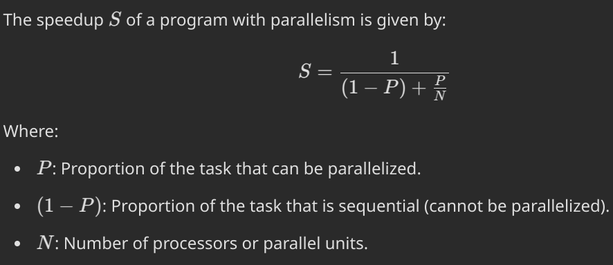The speedup achieved by using parallel computing compared to serial computing depends on how much of the application can run in parallel. For example, if only 30% of the application can be parallelized, even making that part run 100 times faster will only reduce the total execution time by about 29.7%. This means the overall speedup will be about 1.42×. Even if the parallel part becomes infinitely fast, the total speedup will be limited to 1.43×, since 70% of the application still runs sequentially and cannot be improved by parallelization. If 99% of an application’s execution time can run in parallel and the parallel part is made 100× faster, the total execution time will shrink to 1.99% of the original, giving an overall speedup of 50× for the entire application.

the importance of a large portion of an application’s workload being suitable for parallel execution. If the majority of the workload in an application can be parallelized, a multi-processor parallel computing system can be utilized more effectively, leading to significant performance improvements. In short, the larger the parallelizable portion of an application, the greater the speedup that can be achieved from parallel processors.

The achievable speedup also depends on how quickly data can be accessed and written to memory. Direct parallelization often saturates DRAM bandwidth, limiting speedup to about 10×. Overcoming this requires using GPU on-chip memory to reduce DRAM accesses, but further code optimization is needed to address on-chip memory limitations. Additionally the speedup achieved over a single-core CPU reflects how well the CPU suits the application. Some tasks run efficiently on CPUs, making GPU acceleration harder. It’s essential to optimize code so GPUs complement CPU performance, leveraging the strengths of both in heterogeneous computing.

Challenges

Many real-world problems are most naturally described with mathematical recurrences. Parallelizing these problems often requires non intuitive ways of thinking about the problem and may require redundant work during execution.

Memory and Compute Bound Applications: Many applications are memory-bound, meaning their speed is limited by memory access latency/bandwidth or throughput. These require optimization of memory access to achieve better performance. In contrast, compute-bound applications are limited by the number of instructions executed per byte of data. Achieving high-performance parallel execution in memory-bound applications often requires methods for improving memory access speed.

Sensitivity to Input Data: Parallel programs are often more affected by input data characteristics than sequential ones. Problems like varying data sizes or uneven data distributions can lead to an uneven workload across threads, reducing efficiency. These variations can cause significant performance fluctuations. We need to regularize data distributions and/or dynamically refining the number of threads to address these challenges

Synchronization and Collaboration: Some applications, known as embarrassingly parallel, can be easily parallelized with minimal thread collaboration. Others require significant coordination between threads, using synchronization mechanisms like barriers or atomic operations. These operations add overhead, as threads may need to wait for others, reducing efficiency.

Data Parallelism

Example: Grayscale Conversion of Image Weighted Sum

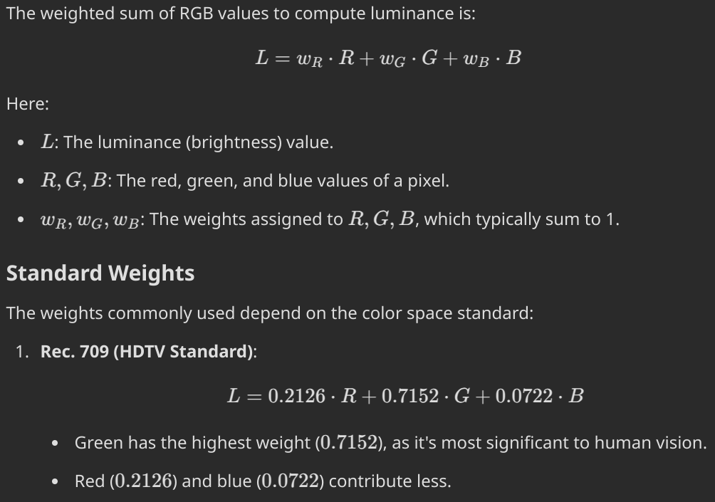
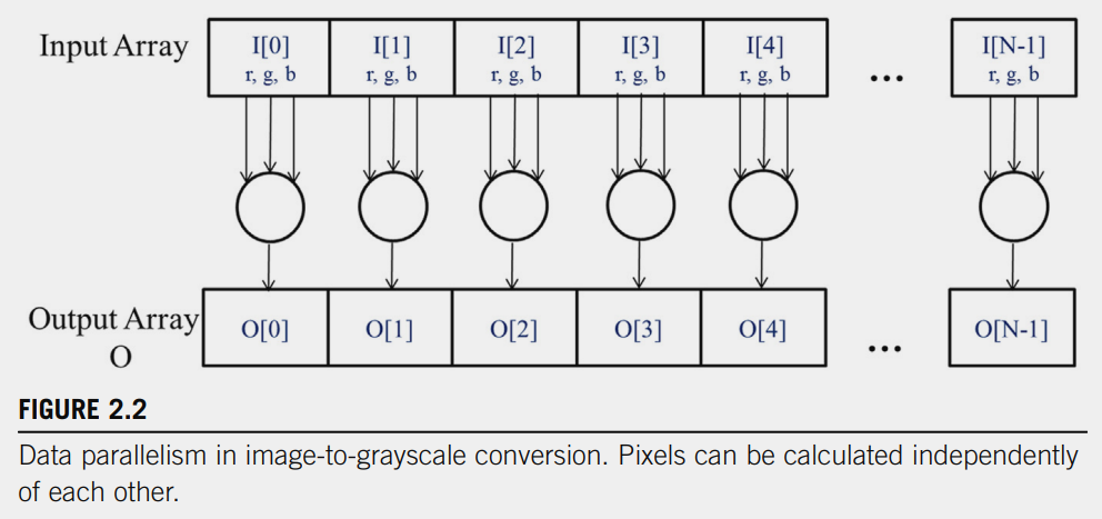
If we think of an input image as an array I containing RGB values, and the output as another array O containing the corresponding luminance values, the process becomes straightforward Each luminance value in O is calculated by taking the weighted sum of the RGB values of the corresponding pixel in I. For example: O[0] is calculated using the RGB values of I[0] O[1] is calculated using the RGB values of I[1] O[2] is calculated using the RGB values of I[2], and so on.

The key point is that each pixel’s computation is independent of the others. This means:

• You can calculate each luminance value (O[i]) without needing to know the results of the other pixels.
• All these calculations can happen in parallel, making the process highly suitable for parallel computing.

Task Parallelism vs. Data Parallelism

Data parallelism is not the only type of parallelism used in parallel programming. Task parallelism has also been used extensively in parallel programming. Task parallelism is typically exposed through task decomposition of applications. For example, a simple application may need to do a vector addition and a matrix-vector multiplication. Each of these would be a task. Task parallelism exists if the two tasks can be done independently. I/O and data transfers are also common sources of tasks. In large applications, there are usually a larger number of independent tasks and therefore larger amount of task parallelism.

CUDA C Program Structure

A CUDA C program combines host (CPU) and device (GPU) code in the same source file. Traditional C code runs on the host, while device code, marked with special CUDA keywords, runs on the GPU. Device code includes functions (kernels) designed for data-parallel execution. 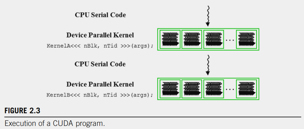(Figure 2.3 shows the simplified execution of two grids of threads and CPU/GPU execution do not overlap)

The execution starts with host code (CPU serial code). When a kernel function is called, a large number of threads are launched on a device to execute the kernel. All the threads that are launched by a kernel call are collectively called a grid. These threads are the primary vehicle of parallel execution in a CUDA platform. When all threads of a grid have completed their execution, the grid terminates, and the execution continues on the host until another grid is launched. Many heterogeneous computing applications manage overlapped CPU and GPU execution to take advantage of both CPUs and GPUs.

Hierarchy in CUDA:

• Thread: The smallest unit that performs the operation.
• Block: The structure in which threads are grouped.
• Grid: The larger structure in which blocks are organized.

In CUDA, each thread and block is addressed by indexes:

• threadIdx: Specifies the index of a thread within a block.
• blockIdx: Specifies the index of a block within the grid.
• blockDim: Specifies the total number of threads within a block.
• Global Index: Used to calculate each thread’s unique index in the array:

How Kernel Functions Work

1. Launch: When the CPU calls a kernel, the GPU creates thousands of threads based on the grid and block configuration.
2. Parallel Execution: Each thread runs the kernel function on its data.
3. Independence: Threads operate independently, but they can share data if needed.

In the color-to-grayscale conversion example, each thread could be used to compute one pixel of the output array O. In this case, the number of threads that ought to be generated by the grid launch is equal to the number of pixels in the image.

Vector Addition Kernel

Vector addition is arguably the simplest possible data parallel computation, the parallel equivalent of “Hello World” from sequential programming. C program that consists of a main function and a vector addition function.

//float A_h[] = {1.0, 2.0, 3.0}; #3
//float B_h[] = {4.0, 5.0, 6.0}; #3
//float C_h[3]; 

// Compute vector sum C_h = A_h + B_h 
// Result: C_h[] = {5.0, 7.0, 9.0}
// Since we have only host code we see only variables suffixed with “_h”.
void vecAdd(float* A_h, float* B_h, float* C_h, int n) { 
	for (int i = 0; i < n; ++i) {
	C_h[i] = A_h[i] + B_h[i];
	}
}
int main() {
// Memory allocation for arrays A, B, and C
// I/O to read A and B, N elements each
	vecAdd(A, B, C, N);
}

In examples, whenever there is a need to distinguish between host and device (CPU) data, we will suffix the names of variables that are used by the host with _h and those of variables that are used by a device (GPU )with _d to remind ourselves of the intended usage of these variables.

A straightforward way to execute vector addition in parallel is to modify the vecAdd function and move its calculations to a device (GPU)

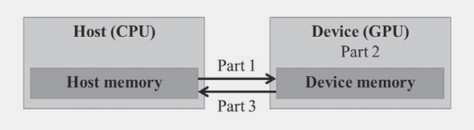
• Part 1 of the function allocates space in the device (GPU) memory to hold copies of the A, B, and C vectors and copies the A and B vectors from the host memory to the device memory.
• Part 2 calls the actual vector addition kernel to launch a grid of threads on the device
• Part 3 copies the sum vector C from the device memory to the host memory and deallocates the three arrays from the device memory.

void vecAdd(float* A, float* B, float* C, int n) {
// Calculate the total memory size required for the vectors (in bytes)
    int size = n * sizeof(float);
// Declare device pointers for the vectors A, B, and C
    float *d_A, *d_B, *d_C;

    // Part 1: Allocate device memory for A, B, and C
    // Copy A and B to device memory
    // ...

    // Part 2: Call kernel – to launch a grid of threads
    // to perform the actual vector addition
    // ...

    // Part 3: Copy C from the device memory
    // Free device vectors
    // ...
}

Revised vecAdd function is essentially an outsourcing agent that ships input data to a device, activates the calculation on the device, and collects the results from the device. The agent does so in such a way that the main program does not need to even be aware that the vector addition is now actually done on a device.

Device Global Memory and Data Transfer

For the vector addition kernel, before calling the kernel, the programmer needs to allocate space in the device global memory and transfer data from the host memory to the allocated space in the device global memory.

Part 1 Similarly, after device execution the programmer needs to transfer result data from the device global memory back to the host memory and free up the allocated space in the device global memory that is no longer needed.

In Part 1 and Part 3 of the vecAdd function need to use the CUDA API functions to allocate device global memory for A, B, and C; transfer A and B from host to device; transfer C from device to host after the vector addition; and free the device global memory for A, B, and C.

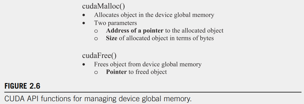
cudaMalloc is a CUDA function used to allocate memory on the GPU’s global memory. It works similarly to the malloc function in C but allocates memory on the GPU instead of the CPU.

cudaMalloc takes two parameters:

1. First Parameter: The address of a pointer that will hold the address of the allocated memory.

   • You need to cast this pointer’s address to (void**) because cudaMalloc is designed to work with pointers of any type.
   • The memory is allocated on the GPU, and the pointer stores the GPU memory address.

2. Second Parameter: The size of the memory to allocate, specified in bytes.

   • For example, if you want an array of n elements of type float, you calculate the total size as -> Memory Size = n x sizeof(float)

float* A_d;                   // Pointer for memory on the GPU
int size = n * sizeof(float); // Calculate memory size in bytes

// Allocate memory on the GPU
cudaMalloc((void**)&A_d, size);

1. float* A_d:

   • This declares a pointer A_d that will point to memory on the GPU.
   • At this point, no memory has been allocated; the pointer is just declared.

2. int size = n * sizeof(float);:

   • This calculates the amount of memory to allocate on the GPU in bytes.
   • If n=1000and the size of float is 4 bytes -> size = 1000x4 = 4000bytes

3. cudaMalloc((void**)&A_d, size);:

   • cudaMalloc allocates 4000 bytes of memory on the GPU.
   • The address of the allocated memory is stored in A_d.

After you’re done with the allocated memory, you should free it using cudaFree:

cudaFree(A_d);

This releases the memory allocated on the GPU.