Onur's CS Journey

Statistical learning is a fundamental concept in the field of data analysis and predictive modeling. At its core, it encompasses a collection of methodologies and algorithms aimed at estimating a function f, which represents the relationship between a set of inputs and corresponding outputs. This process enables us to understand patterns in data, make predictions, and derive actionable insights from complex datasets. By leveraging statistical principles, mathematical models, and computational techniques, statistical learning bridges theory and application, serving as a cornerstone for modern data science and machine learning.

Input Variable

The input variables in other words the data provided to the model to make predictions or decision are typically represented using the symbol X, with subscripts to distinguish between them, such as X₁, X₂, X₃, and so on. These inputs are referred to by various terms, including:

Predictors
Independent variables
Features
Variables

Output Variable

The output variable, often called the response or dependent variable, is usually represented by the symbol Y. This variable represents the outcome or the target the model aims to predict or understand.

In a more general context, suppose we observe a quantitative response Y and P different predictors (X₁, X₂, …, Xₚ). We assume that there exists a relationship between Y and X = (X₁, X₂, …, Xₚ), which can be expressed in a general form as:

$$ Y = f(X) + \epsilon $$

Here:

f(X) represents the true underlying relationship between the predictors and the response.
ε denotes the error term, which is independent of X and has mean zero. The error term also accounts for variability in Y that cannot be explained by f(X).

Error Term

Prediction

In many scenarios, a set of inputs $X$ is readily available, but the output $Y$ cannot be easily obtained. In such cases, we can predict $Y$ using the equation:

$$ \hat{Y} = \hat{f}(X), $$

where $\hat{f}$ represents our estimate of the function $f$, and $\hat{Y}$ denotes the resulting prediction for $Y$. Since the error term averages to zero, this approach allows for reasonable predictions. Notably, $\hat{f}$ is often treated as a “black box,” meaning that the exact form of $\hat{f}$ is not typically a concern, as long as it produces accurate predictions for $Y$.

The accuracy of $\hat{Y}$ as a prediction for $Y$ depends on two components: reducible error and irreducible error.

Reducible Error: The estimate $\hat{f}$ may not perfectly capture the true function $f$, leading to some error. This error is reducible because it can potentially be minimized by selecting the most appropriate statistical learning technique to estimate $f$.
Irreducible Error: Even if we could form a perfect estimate of $f$, such that our prediction takes the form $\hat{Y} = f(X)$, the prediction would still have some error. This is because $Y$ also depends on $\epsilon$, the error term, which by definition cannot be predicted using $X$. The variability associated with $\epsilon$ contributes to the irreducible error, which cannot be eliminated regardless of how well $f$ is estimated.

Decomposition of Error

The decomposition of the error can be expressed as:

$$ \mathbb{E}[(Y - \hat{Y})^2] = \mathbb{E}[(f(X) + \epsilon - \hat{f}(X))^2] $$

$$ = [f(X) - \hat{f}(X)]^2 + \text{Var}(\epsilon). $$

Expected Prediction Error $\mathbb{E}[(Y - \hat{Y})^2]$: This term represents the average squared difference between the predicted value ($\hat{Y}$) and the actual value ($Y$). It quantifies the overall error in the predictions made by the model.
Reducible Error $[f(X) - \hat{f}(X)]^2$: This term measures the error due to the model’s inability to perfectly estimate the true function $f(X)$. It depends on how well the statistical learning method can approximate $f$. The reducible error can be minimized by improving the model.
Irreducible Error ($\text{Var}(\epsilon)$): This term represents the variability in $Y$ that cannot be explained by the predictors $X$. It arises from $\epsilon$, the error term, which is independent of $X$ and has mean zero. The irreducible error sets a fundamental limit on the accuracy of any prediction model, as it cannot be reduced regardless of how well $f$ is estimated.

Inference

We are often interested in understanding the association between $Y$ and $X_1, \dots, X_p$. In this situation, we aim to estimate $f$, but our goal is not necessarily to make predictions for $Y$. Here, $\hat{f}$ cannot be treated as a black box because we need to understand its exact form. Inference try to answer questions like:

Which predictors are associated with the response?
What is the relationship between the response and each predictor?
Can the relationship between $Y$ and each predictor be adequately summarized using a linear equation, or is the relationship more complicated?

How to Estimate $f$

We will always assume that we have observed a set of $n$ different data points. These observations are called the training data because we use them to train, or teach, our method how to estimate $f$.

Let $x_{ij}$ represent the value of the $jth$ predictor (or input) for the $ith$ observation, where $i = 1, 2, \dots, n$ and $j = 1, 2, \dots, p$. Correspondingly, let $y_i$ represent the response variable for the $ith$ observation. Then, our training data consist of:

$$ {(x_1, y_1), (x_2, y_2), \dots, (x_n, y_n)} $$ where:

$$ x_{i} = (x_{i1}, x_{i2}, \dots, x_{ip})^\top $$

is the vector of predictors for the $ith$ observation. Our goal is to apply a statistical learning method to the training data in order to estimate the unknown function $f$. In other words, we want to find a function $\hat{f}$ such that:

$$ Y \approx \hat{f}(\mathbf{X}) $$

for any observation $(\mathbf{X}, Y)$. Most statistical learning methods for this task can be characterized as either parametric or non-parametric

Parametric Methods

Parametric methods use a two-step process to estimate the relationship between the predictors ($X$) and the response ($Y$).

Step 1: Assume the Shape of $f$ First, we make an assumption about the form of the function $f$ that links $X$ and $Y$. A common assumption is that $f$ is linear, meaning: $$ f(X) = \beta_0 + \beta_1X_1 + \beta_2X_2 + \cdots + \beta_pX_p $$ Here:

$\beta_0$ is the intercept.
$\beta_1, \beta_2, \dots, \beta_p$ are the coefficients that measure the effect of the predictors ($X_1, X_2, \dots, X_p$) on $Y$.

By assuming a linear form, we simplify the problem. Instead of estimating a complex, unknown function $f$, we only need to estimate a few parameters: $\beta_0, \beta_1, \dots, \beta_p$.

Step 2: Fit the Model Next, we use data to “fit” the model, meaning we find the best values for $\beta_0, \beta_1, \dots, \beta_p$ so that: $$ Y \approx \beta_0 + \beta_1X_1 + \beta_2X_2 + \cdots + \beta_pX_p $$

The most common method for fitting the model is Ordinary Least Squares works by finding the values of $\beta_0, \beta_1, \dots, \beta_p$ that minimize the difference between the predicted values ($\hat{Y}$) and the actual values ($Y$).

Advantages:

By assuming a specific form for $f$ (e.g., linear), parametric methods reduce the problem to estimating a small number of parameters, making the process straightforward.
With fewer parameters to estimate, parametric methods work well even with smaller datasets.

Disadvantages:

If the assumed form of $f$ (e.g., linear) is very different from the true relationship, the model will give poor predictions.
Parametric models are less flexible and may struggle to capture complex patterns in the data.

Flexibility vs. Overfitting

To address the limitations, we can use more flexible models that can fit a wider variety of patterns. However:

Flexible models often require estimating more parameters.
More complex models may overfit, meaning they fit the noise in the data rather than the true pattern, leading to poor performance on new data.

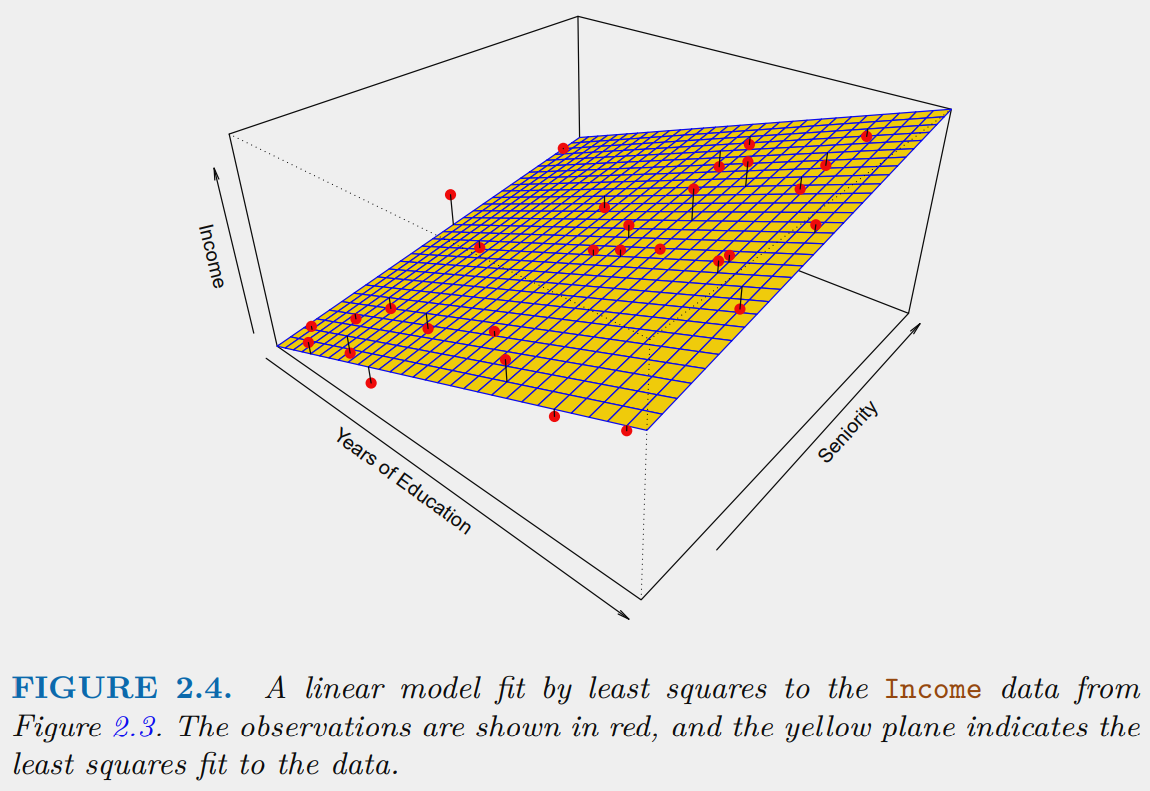
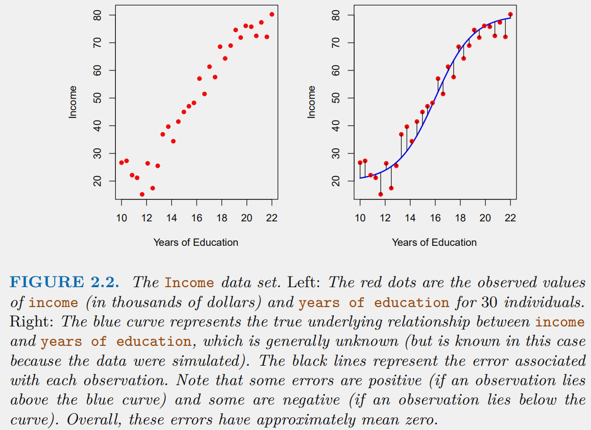
Example: Income Data

We have fit a linear model of the form: $$ \text{income} \approx \beta_0 + \beta_1 \times \text{education} + \beta_2 \times \text{seniority}. $$

Linear Fit

Statistical Learning